

Your Success, Our Mission!
6000+ Careers Transformed.
Explanation:
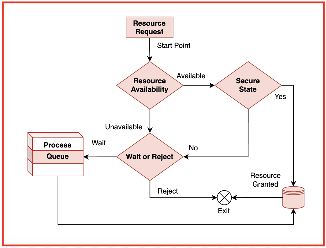
Banker’s Algorithm is a deadlock avoidance algorithm used by Operating Systems to ensure that resource allocation always keeps the system in a safe state. The name “banker” comes from its resemblance to how a banker manages loans: a banker will only grant a loan if doing so does not prevent all customers from eventually repaying. In the same way, the OS grants resources only if doing so allows all processes to complete without entering deadlock.
The algorithm is needed because many real-world applications request resources unpredictably during execution. If the OS blindly allocates resources, the system may transition into an unsafe state, eventually leading to deadlock. Banker’s Algorithm proactively checks whether granting a request maintains system safety.
Example:
If a process requests additional memory pages, the OS evaluates:
• “If I allocate now, will I still have enough to satisfy all other processes later?”
If yes → safe allocation
If no → request is delayed
Reason | Explanation |
| Avoid unsafe states | Prevent deadlocks before they occur |
| Manage dynamic requests | Processes change demands at runtime |
| Ensure fairness | Every process gets a chance to finish |
| Maintain OS stability | Predictable system behavior |
Use Cases:
• Multiprogramming OS requiring strict control over resource allocation
• Banking, financial, or trading systems needing strict consistency
• Real-time applications where safety is more important than speed
Explanation:
Although Banker’s Algorithm is theoretically powerful, it is rarely used in real-time systems because of strict timing constraints. Real-time applications require guaranteed worst-case execution time, which Banker’s Algorithm cannot provide due to:
• Dynamic checking of multiple states
• Matrix scanning for safe sequence
• High computational overhead
• Need for complete resource usage predictions
Real-time systems often rely on static resource reservation, priority scheduling, or lock-free algorithms instead of Banker’s Algorithm.
Example:
A real-time medical monitoring system cannot delay resource allocation just to compute safe states.
Limitation | Reason |
| High overhead | Matrix operations every request |
| Needs maximum future demands | Hard to predict in real-time |
| Possible delays | Violates strict timing constraints |
Use Cases:
• Aerospace real-time controls
• Medical embedded systems
• Automotive control units

Explanation:
Allocation Matrix stores the number of each resource type currently allocated to every process. It represents the current state of resource distribution in the system.
Example Matrix:
Process A B C
P0 0 1 0
P1 2 0 0
P2 3 0 2
Purpose | Description |
| Track resource ownership | Shows how many resources each process holds |
| Used in safe-state calculation | Determines if processes can finish |
| Required by request algorithm | Ensures safe allocation |
Use Cases:
• Tracking OS-level resource assignment
• Detecting resource bottlenecks
• Predicting safe completion sequences

Explanation:
Maximum Matrix indicates the maximum number of each resource type each process may request during execution. It helps the algorithm plan future resource usage safely.
Example Matrix:
Process A B C
P0 7 5 3
P1 3 2 2
P2 9 0 2
Use Cases:
• Ensuring that future resource demands remain satisfiable
• Preventing overcommitment of system resources
• Checking safe state transitions

Explanation:
Need Matrix is derived as:
Need = Max – Allocation
It shows remaining resources required by each process to complete execution.
Example Calculation:
Max (P0): [7 5 3]
Allocation (P0): [0 1 0]
Need = [7 4 3]
Example Matrix:
Process A B C
P0 7 4 3
P1 1 2 2
P2 6 0 0
Use Cases:
• Safe sequence evaluation
• Preventing unsafe state transitions
• Planning for resource reservation

Explanation:
Available Vector stores the number of free resources of each type. It directly influences whether a process can immediately proceed.
Example:
Available Vector:
A: 3, B: 3, C: 2
Resource Type | Available |
| A | 3 |
| B | 3 |
| C | 2 |
Use Cases:
• Checking if demand of a process can be satisfied
• Step 1 of safety algorithm
• Determines system’s immediate capacity

Explanation:
Work Vector represents the currently available resources during safe state analysis. Initially, it is equal to the Available Vector. As processes are assumed to complete, Work is updated by adding their Allocations.
Example:
Available = [3 3 2]
Work = [3 3 2] (initially)
After P1 completes with Allocation [2 0 0]:
Work becomes [5 3 2].
Step | Work Vector |
| Initial | [3 3 2] |
| After P1 completes | [5 3 2] |
Use Cases:
• Safety sequence generation
• Simulating process completion
• Avoiding deadlock-prone allocations

Explanation:
The safe sequence ensures that processes can finish one by one without causing deadlock. A process can finish if its Need ≤ Work. After it completes, its allocated resources are added back to Work.
Example:
Safe sequence found: P1 → P3 → P0
Process | Need | Work Check | Can Execute? |
| P1 | ≤ Work | Yes | Added to sequence |
| P3 | ≤ New Work | Yes | Added |
| P0 | ≤ Final Work | Yes | Completed |
Use Cases:
• Resource allocation validation
• Scheduling optimization
• Transaction ordering

Explanation:
Let Available = [3 3 2]
Allocation Matrix:
P0 0 1 0
P1 2 0 0
P2 3 0 2
Maximum Matrix:
P0 7 5 3
P1 3 2 2
P2 9 0 2
Need Matrix (Max – Allocation):
P0 7 4 3
P1 1 2 2
P2 6 0 0
Process Execution:
Safe Sequence:
P1 → P2 → P0
Order | Process | Work Before | Work After |
| 1 | P1 | [3 3 2] | [5 3 2] |
| 2 | P2 | [5 3 2] | [8 3 4] |
| 3 | P0 | [8 3 4] | [8 4 4] |
Use Cases:
• Teaching deadlock avoidance
• Validating multi-resource scheduling
• OS kernel-level resource planning

Top Tutorials

CNN in Deep Learning 2026
A beginner-friendly guide to CNNs: understand deep learning essentials, create Python-based models, and explore advanced applications.

Breaking The Limits: Scaling Databases with MySQL Partitioning
Learn MySQL partitioning with examples. Improve query performance, scalability, and data management using RANGE, LIST, HASH, KEY, and composite techniques.

ML in Action: Hands-On Guide to Deploying and Serving Models
Learn model deployment and serving—from concepts to real-world architectures, tools, APIs, containers, and cloud workflows for production-ready ML.

 in Bengaluru, India



All Courses (6)
Master's Degree (2)
Fellowship (2)
Certifications (2)

 Idea and Objective


 in Bengaluru, India